
Companies all over the world are increasingly utilizing recommender systems. These systems can be used by online stores, streaming services, or social networks to recommend items to users, based on their previous behavior on a certain platform (either consumed items or searched items), in order to greatly improve the value of the resource.
There are several approaches to developing recommendation systems. One can build a recommender system based on the content of the items to be recommended (its intrinsic features), so that the system will suggest items similar to the ones the user usually likes (Content-Based recommender systems), or we can use similarity metrics to recommend items that other users similar to the one who will receive the suggestions have already rated highly (Collaborative-filtering recommender systems). Collaborative-Filtering (CF) is what we decided to implement for the beginning stages of this project.
To the best of our knowledge, recommender systems are yet to be used in our sector, so we’re aiming to develop cutting-edge technology for the sake of boosting our overall product’s quality. In this post I’ll give a general overview of what we did when conceiving iSolutions’s very first machine learning project, based on Collaborative-Filtering, and the challenges we faced.
Our final objective is to implement a machine learning module, built on top of iSBets, which will provide our customers’ websites with a slicker, more comfortable final user experience for players… But what exactly do we mean by this, and how can this be achieved?
In practice, the end result will consist of a “Match and Odds Recommender”: a section on our betting websites dedicated to personalized suggestions for the final user, tailored around his/her betting preferences, which will consist of a list of matches and markets which the model thinks the user will most likely be willing to bet on. So this not only will reduce the time a user takes on average to get to the portion of the website he desires in order to play, but mainly increases user’s fidelity towards the website, driven by product ease of use and customer appreciation demonstrated by the personalized online experience. Of course this will bring benefits to the bookmakers as well: a satisfied customer is a happy customer, and a happy customer is a returning customer, and this of course has the potential to spur larger profits driven by potentially increased website visits and churn drop.
Now let’s take a quick overview at what we’re doing. Of course the starting point of every machine learning project is data gathering: we extracted thousands of data points relating to dedicated user traffic on our internal test websites and their preferred betting behaviors. We then preprocessed this data with a data transformation pipeline in order to feed it to the CF algorithm. This data needs to be in a specific format, so let’s see why while explaining the model used as well (this is going to take a bit of math, so bare with me):
The technique we used, Singular Value Decomposition (SVD), is a method from linear algebra that has been generally used as a dimensionality reduction technique in machine learning. SVD is a matrix factorization technique, which reduces the number of features of a dataset by reducing the space dimension from N-dimension to K-dimension (where K<N). In the context of the recommender system, the SVD is used as a CF technique. It uses a matrix structure where each row represents a user, and each column represents an item. The elements of this matrix are the ratings that are given to items by users.

The factorization of this matrix is done by the singular value decomposition. It finds factors of matrices from the factorization of a high-level (user-item-rating) matrix. The singular value decomposition is a method of decomposing a matrix into three other matrices: where A is a m x n utility matrix, U is a m x r orthogonal left singular matrix, which represents the relationship between users and latent factors, S is a r x r diagonal matrix, which describes the strength of each latent factor and V is a r x n diagonal right singular matrix, which indicates the similarity between items and latent factors. The latent factors here are the characteristics of the items, for example, the genre of a song or movie. The SVD decreases the dimension of the utility matrix A by extracting its latent factors. It maps each user and each item into a r-dimensional latent space. This mapping facilitates a clear representation of relationships between users and items. The input for this algorithm must of course then be a matrix, which is derived from a Dataset comprised of n rows, each containing three features: a user, an item, and the score that user has assigned to that item.
Let each item be represented by a vector xi and each user is represented by a vector yu. The expected rating by a user on an item rui can be given as:

Here, rui is a form of factorization in singular value decomposition. The xi and yu can be obtained in a manner that the square error difference between their dot product and the expected rating in the user-item matrix is minimum. It can be expressed as: In order to let the model generalize well and not overfit the training data, a regularization term is added as a penalty to the above formula. In order to reduce the error between the value predicted by the model and the actual value, the algorithm uses a bias term. Let for a user-item pair (u, i), μ is the average rating of all items, bi is the average rating of item i minus μ and bu is the average rating given by user u minus μ, the final equation after adding the regularization term and bias can be given as:
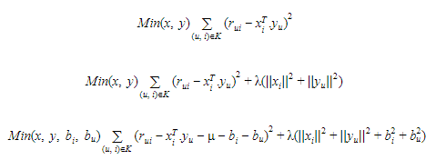
The above equation is the main component of the algorithm which works for singular value decomposition based recommendation system.
So, now that we have factorized, and hence “filled in” our original matrix, we can compute similarity scores between users (or items) in order to segment them and identify which ones are most similar to the one we’ll have to provide the suggestions to. I won’t go into detail with the similarity measures, as not to bore you with more math, if you’re interested you can check out this paper: “Similarity measures for Collaborative Filtering-based Recommender Systems: Review and experimental comparison”. The chosen similarity metric will then let us pick from best rated items a user has between the ones he did not interact with yet, and suggest them, finally, to the user. Of course, in our case, this is not the end of it: our final suggested items are matches and odds, but these both change constantly during time, so the final step is to check the current Event Program against what the system has suggested and recommend only what is available on site right now.
Now, we have run some tests internally utilizing these techniques and have some results to show for it, however, the population taking part in these tests was not very large, so the numbers may not be statistically significative or reflect the truth values for a larger population; at any rate, these are an amazing starting point for this journey and can propel the project moving forward. In the future, when the system will be fully deployed, we’ll have access to a larger dataset for our measurements and the evaluations will surely be more significant. Let’s see what we found out: first of all, we tried taking a look at the overall trend of funds and times played during the whole duration of our experiment (graph below, grouped by week, normalized).
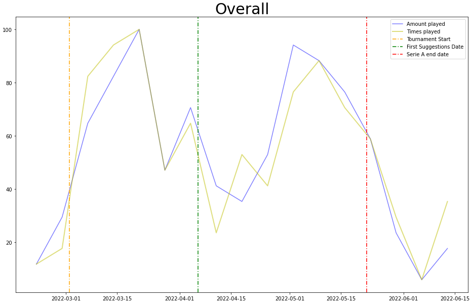
As you can see, the progression is kind of erratic, and it’s difficult to say whether the suggestions affect the behavior on site or not. This is because the players are influenced by a myriad of factors beyond the suggestions, for example: what games are available during a specific week, how many funds the player has available to bet, if the players feel like betting at all, and many possible more. So where can we go from here? Well, let’s take a look at the conversion rates, that is to say if a player decided to play a match we suggested (graph below, grouped by week) .
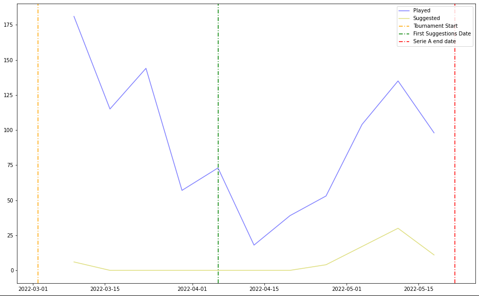
Here, the blue line represents the number of games played each week, and the yellow line represents the number of games that were suggested by the algorithm and also played by users. From this, we can tell a couple of things: it may seem that the conversion rate is not really significant compared to the total played, but let’s take a closer dive. The model is still a prototype and it has been evolving constantly during the course of this experiment and gotten consistently better and bigger (comprising of more features), true, unfortunately the process with which we advanced along all the duration of the measurements has not been fast and reactive as much as it could have been since everything was done by hand (from data extraction to model training), hence the prediction may not have been up to par or anyway as good as they could have been. However, an hidden parameter may show a LOT of promise going forward: the correlation between the two measures.
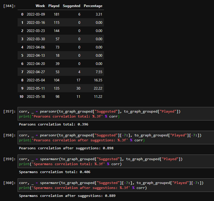
Let’s have a look at the two parts of this image: first, a Dataset clearly showing the conversion rates for each week (suggestions started after index ‘4’). The more the users play, the more the conversion rate percentage goes up; this could mean that our predictions were often correct, and the more the userbase plays, the more this is caught and shown in the conversion rate. The most interesting point we can extract from this analysis however, as we anticipated, is the actual correlation between the two measures. Shown in the second part of the image, are the raw values an they are sky high! This can mean that the more the users play, the more the suggestions are revealed to be correct and taken into consideration by the players. This is vital to our project since if the correlations would have been close to 0 we would have had proof that our suggestions were totally incorrect and/or ignored.
Going forward, we want to implement new features inside the algorithm itself, but also integrate it with the current structure of iSBets, by building automated pipelines and UIs for starters, in order to be more accurate during the prediction step and also be more user-friendly, always trying to get closer and closer to our final objective of having more satisfied users and clients.
Thank you for taking the time to read this post, explaining the introduction into the world of Artificial Intelligence for iSolutions.
Many more interesting projects are yet to come!